Returns vs. 10-K Sentiment

By: Taylor Sheridan

Summary

This report aims to answer the question of whether the positive or negative sentiment in a 10-K is associated with better/worse stock returns. In order to explore this question, I followed the steps listed below:

Downloaded data on sp500 companies from wikipedia
Download each firm’s 2022 10-K file and put them in a zip folder
Clean and store each 10-K’s html text
Create positive/negative sentiment dictionary, as well as contextual sentiment topic lists
Use regex function to create sentiment scores for each firm’s 10-K
Use CIK and accession number to grab the filing date of each firm’s 10-K
Download 2022 stock returns
Merge sentiment dataset with return dataset on symbol and filing date
Download 2021 ccm accounting data
Merge ccm dataset on Symbol to create dataset for analysis

After I collected my data and created a master dataset, I explored the relationships between a firm’s stock returns on its 10-K filing date and the sentiment of its 10-K. From my findings, I discovered very weak relationships between stock returns and sentiment scores. This has mostly to do with incomplete data which I will explain within the data section of this report. However, I still managed to gain some insights into this relationship.

Data

The sample used for this analysis is firms within the sp500. Using the steps listed above, each firm’s return on its 10-K filing date was added to the dataset, as well as sentiment variables using a regex function. Finally, this data was combined with ccm accounting data for additional firm statistics.

The intended return variables for this assignment were to capture firm returns 2 days after the 10-K release, and returns between day 3-10 after the release. Unfortunately, I was unable to accomplish this, but below is my code to grab cumulative firm returns:

analysis_df['cum_ret'] = analysis_df.assign(RET=1+clean_df['ret']).groupby('Symbol')['RET'].cumprod()

This is only the code to get the cumulative returns for each firm, which would be the first step, but I was unable to figure out how to grab the returns for those two time periods around the 10-K filing date and store them in a new variable. I assume .transform() would have been useful.

The next step was to create sentiment variables for each firm’s 10-K. I created 10 variables to score the file’s positive or negative sentiment, as well as sentiment towards certain topics. Below is an example of how I created one of the sentiment variables, ‘ML_Negative’, which is sentiment using a list of negative words derived from machine learning:

with open('inputs/ML_negative_unigram.txt', 'r') as myfile:
    BHR_negative = [line.strip() for line in myfile]                # creates negative word list
    
    
BHR_negative_regex = '(' + '|'.join(BHR_negative) + ')'             # formats properly for regex function
regex1 = NEAR_regex([BHR_negative_regex])`                          # insert into regex function

for index, row in tqdm(firms_df1.iterrows()):                       # for loop for all firms
        
    doc_length = len(row['clean_html'].split())                     # stores length of file
        
    ML_negative_words = len(re.findall(regex1, row['clean_html']))  # finds all negative words from list within file
    BHR_negative_score = ML_negative_words / doc_length             # divide by length to get score
    firms_df1.loc[index, 'ML_Negative'] = BHR_negative_score        # store in variable

In addition to the positive/negative sentiment scores, I chose to explore how 3 topics were discussed within each 10-K to see if those individual topics affected stock price movement more. The three topics I chose were “covid”, “inflation”, and “innovation.” I chose these topics because I thought they were relevant to business and the state of our economy. Covid-19 has been a hot topic of discussion in recent years because of its threat to people’s lives, which both directly and indirectly affects business. I expected discussion on covid to have a negative impact on stock price. I also chose inflation because the rise of interest rates has greatly affected the economy and companies are monitoring them closely to predict its future impact. I expected discussion on inflation to decrease stock price, but not by much. Finally, I chose innovation because companies are always looking to make positive change and become a front-runner in their respective industries. I anticipate conversation around innovation to have a positive impact on stock performance.

I provided a table of summary statistics of my final analysis sample below:

import pandas as pd
pd.options.display.max_columns = None
pd.options.display.max_rows = None

analysis_df = pd.read_csv('output/analysis_sample.csv')
analysis_df.describe()

	CIK	ML_Negative	ML_Positive	LM_Negative	LM_Positive	Covid_Negative	Covid_Positive	Inflation_Negative	Inflation_Positive	Innovation_Negative	Innovation_Positive	ret	gvkey	fyear	lpermno	lpermco	sic	sic3	td	long_debt_dum	me	l_a	l_sale	capx_a	div_d	age	atr	smalltaxlosscarry	largetaxlosscarry	gdpdef	l_reala	l_reallongdebt	kz_index	ww_index	hp_index	ww_unconstrain	ww_constrained	kz_unconstrain	kz_constrained	hp_unconstrain	hp_constrained	tnic3tsimm	tnic3hhi	prodmktfluid	delaycon	equitydelaycon	debtdelaycon	privdelaycon	at_raw	raw_Inv	raw_Ch_Cash	raw_Div	raw_Ch_Debt	raw_Ch_Eqty	raw_Ch_WC	raw_CF	l_emp	l_ppent	l_laborratio	Inv	Ch_Cash	Div	Ch_Debt	Ch_Eqty	Ch_WC	CF	td_a	td_mv	mb	prof_a	ppe_a	cash_a	xrd_a	dltt_a	invopps_FG09	sales_g	dv_a	short_debt
count	4.040000e+02	404.000000	404.000000	404.000000	404.000000	404.000000	404.000000	404.000000	404.000000	404.000000	404.000000	404.000000	296.000000	296.0	296.000000	296.000000	295.000000	295.000000	296.000000	296.0	2.960000e+02	296.000000	296.000000	296.000000	296.000000	296.000000	296.000000	225.000000	225.000000	296.000000	296.000000	296.000000	275.000000	295.000000	296.000000	296.000000	295.000000	296.000000	275.000000	296.0	296.0	261.000000	261.000000	259.000000	0.0	0.0	0.0	0.0	296.000000	296.000000	296.000000	296.000000	296.000000	296.000000	296.000000	296.000000	296.000000	296.000000	296.000000	296.000000	296.000000	296.000000	296.000000	296.000000	296.000000	296.000000	296.000000	296.000000	296.000000	296.000000	296.000000	296.000000	296.000000	296.000000	277.000000	295.000000	296.000000	296.000000
mean	7.911027e+05	0.026199	0.024079	0.016107	0.005046	0.000431	0.000182	0.000269	0.000142	0.000911	0.000686	0.167894	43783.293919	2021.0	53033.912162	26228.320946	4277.701695	427.545763	14267.287520	1.0	9.182268e+04	9.980973	9.506013	0.029643	0.746622	1.986486	0.212397	0.711111	0.226667	121.574561	5.180524	3.904354	-6.637216	-0.352671	-2.690920	0.787162	0.088136	0.351351	0.214545	1.0	0.0	3.767452	0.325586	3.203900	NaN	NaN	NaN	NaN	41881.764321	0.065606	-0.009950	0.023712	0.008183	-0.046383	0.017259	0.117568	3.343312	8.107116	4.823714	0.065606	-0.009950	0.023712	0.007255	-0.044298	0.015921	0.117568	0.349147	0.181725	3.480484	0.153559	0.231585	0.133054	0.028327	0.321326	3.128103	0.291556	0.023712	0.089924
std	5.569934e+05	0.003227	0.003492	0.003711	0.001354	0.000259	0.000124	0.000162	0.000094	0.000302	0.000221	3.584079	59711.952251	0.0	30077.168794	16824.282114	1945.905139	194.622792	23043.292915	0.0	2.390276e+05	1.108001	1.194087	0.024414	0.435682	0.141971	0.182540	0.454257	0.419609	1.533136	1.107450	1.292392	8.495044	0.336028	0.314564	0.410007	0.283974	0.478201	0.411255	0.0	0.0	9.033720	0.272094	1.737992	NaN	NaN	NaN	NaN	64008.097754	0.089279	0.055106	0.025755	0.084213	0.067102	0.062267	0.087549	1.096886	1.438016	1.346984	0.089279	0.055106	0.025755	0.077423	0.059943	0.048565	0.087549	0.189848	0.143796	2.747725	0.083325	0.203483	0.122334	0.042566	0.183141	2.784793	0.868479	0.025755	0.089011
min	2.488000e+03	0.008953	0.003546	0.006875	0.001773	0.000000	0.000000	0.000000	0.000000	0.000000	0.000000	-24.277852	1045.000000	2021.0	10104.000000	7.000000	100.000000	10.000000	60.067000	1.0	6.559703e+03	7.592752	6.836294	0.001387	0.000000	0.000000	0.000000	0.000000	0.000000	117.922000	2.791126	0.329143	-50.967920	-0.647860	-3.230299	0.000000	0.000000	0.000000	0.000000	1.0	0.0	1.000000	0.036273	0.457329	NaN	NaN	NaN	NaN	1983.764000	-0.239829	-0.324262	0.000000	-0.206671	-0.357998	-0.150786	-0.613519	0.625938	4.580744	0.519750	-0.239829	-0.324262	0.000000	-0.206671	-0.223117	-0.150786	-0.613519	0.006418	0.000676	0.878375	-0.077358	0.013654	0.004218	0.000000	0.004913	0.481436	-0.658981	0.000000	0.000000
25%	9.767775e+04	0.024186	0.021882	0.013652	0.004092	0.000242	0.000094	0.000153	0.000073	0.000702	0.000541	-1.618724	6420.000000	2021.0	19474.750000	13972.750000	2843.000000	284.000000	3256.413000	1.0	1.900649e+04	9.250529	8.636038	0.012694	0.000000	2.000000	0.125560	0.000000	0.000000	121.708000	4.461192	3.201480	-10.787620	-0.495996	-2.929592	1.000000	0.000000	0.000000	0.000000	1.0	0.0	1.101900	0.130472	2.006005	NaN	NaN	NaN	NaN	10410.080000	0.021447	-0.031603	0.000000	-0.029409	-0.068264	-0.003505	0.069272	2.555745	7.054157	4.001654	0.021447	-0.031603	0.000000	-0.029409	-0.068264	-0.003505	0.069272	0.227240	0.072934	1.647529	0.099179	0.089342	0.041530	0.000000	0.200364	1.350073	0.085556	0.000000	0.026400
50%	8.853060e+05	0.026048	0.024150	0.015948	0.004957	0.000380	0.000152	0.000241	0.000121	0.000866	0.000662	-0.096874	13710.500000	2021.0	57737.000000	21169.000000	3728.000000	372.000000	6772.000000	1.0	3.463996e+04	9.917810	9.440016	0.022716	1.000000	2.000000	0.193019	1.000000	0.000000	121.708000	5.116185	3.938389	-3.761360	-0.457291	-2.725088	1.000000	0.000000	0.000000	0.000000	1.0	0.0	1.363700	0.236235	2.883351	NaN	NaN	NaN	NaN	20288.500000	0.044525	-0.003761	0.017509	-0.001578	-0.023804	0.009987	0.106095	3.246491	8.046027	4.530496	0.044525	-0.003761	0.017509	-0.001578	-0.023804	0.009987	0.106095	0.321847	0.153236	2.535912	0.137471	0.158500	0.097425	0.009919	0.299592	2.170944	0.158671	0.017509	0.061669
75%	1.136875e+06	0.028200	0.026164	0.018106	0.005801	0.000572	0.000252	0.000347	0.000188	0.001068	0.000806	1.798563	61435.750000	2021.0	82546.750000	40395.750000	5331.000000	533.000000	14422.000000	1.0	7.192174e+04	10.702927	10.170132	0.038324	1.000000	2.000000	0.235804	1.000000	0.000000	121.708000	5.891841	4.667277	-0.574875	-0.378925	-2.507755	1.000000	0.000000	1.000000	0.000000	1.0	0.0	2.140700	0.432629	4.150276	NaN	NaN	NaN	NaN	44485.916000	0.084956	0.013003	0.037061	0.020383	-0.000694	0.026170	0.161380	4.191917	9.094283	5.453990	0.084956	0.013003	0.037061	0.020383	-0.000694	0.026170	0.161380	0.445578	0.245099	4.285134	0.197564	0.309560	0.179042	0.041274	0.405472	3.701127	0.290145	0.037061	0.123019
max	1.868275e+06	0.038030	0.037982	0.030185	0.010899	0.001429	0.000793	0.001075	0.000603	0.002026	0.001557	16.214105	316056.000000	2021.0	93132.000000	58235.000000	8742.000000	874.000000	177930.000000	1.0	2.324390e+06	12.949316	13.253324	0.157599	1.000000	2.000000	1.000000	1.000000	1.000000	126.907000	8.147692	7.222624	3.794306	1.055742	-1.802074	1.000000	1.000000	1.000000	1.000000	1.0	0.0	80.969100	1.000000	11.815062	NaN	NaN	NaN	NaN	420549.000000	0.586530	0.171227	0.163095	0.734575	0.133418	0.780077	0.552110	5.247024	10.627358	9.737904	0.586530	0.171227	0.163095	0.460031	0.133418	0.390622	0.552110	1.161385	0.798769	14.733148	0.405925	0.888302	0.607837	0.258595	1.019505	14.066011	14.183099	0.163095	0.530059

After taking a first look at my data and some analysis, I did not notice anything unusual; however, this is because I understand my data is incomplete and this will be explained below. One thing I would point out is how low my sentiment scores are. This likely means that either my topics did not receive a lot of hits, or I made an error.

Data Warning !!!

When assembling my data, I ran into a few issues that greatly impacted the results of my analysis. The most significant error is that I was not able to get return variables for each firm 2 days after the 10-K filing, and 3-10 days after. I only used the firm’s returns on that day of trading. This would have been sufficient to identify some relationship between stock returns and 10-K sentiment, but 10-K’s are released at different times of day, meaning the return on that day can be caused by many different factors. For example, a firm may not release their 10-K until 4pm, but trading is already finished, so the returns in my data are not related to the 10-K sentiment, other than insider trading, rumors, etc…

Another problem with my data is that it only represents 405 firms in the sp500. When downloading each firm’s 10-K html file, I only grabbed 405, and so I dropped the rest. I still belive 80% of the population would be enough to make some kind of conclusion about the relationship, but it wouldn’t be as complete or accurate, especially if some of the top firms were missing.

Results

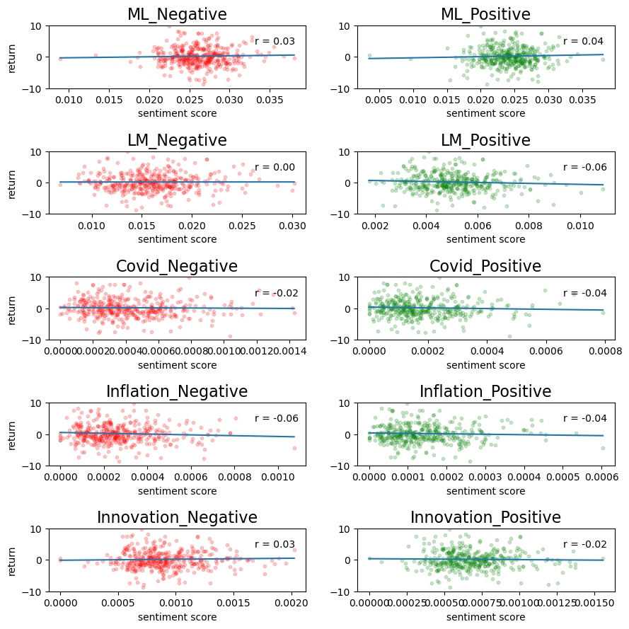
In order to analyze the relationship between a firm’s stock return on its 10-K filing date and the sentiment of its 10-K, I created scatterplots of return vs. sentiment score. I also included correlation coefficients on each graph to describe the strength of the relationship. The code I wrote and its output is provided below:

import pandas as pd
import numpy as np
import seaborn as sns
import matplotlib.pyplot as plt 

analysis_df = pd.read_csv('output/analysis_sample.csv')
a1 = analysis_df[['Symbol','ret','ML_Negative','ML_Positive','LM_Negative','LM_Positive','Covid_Negative','Covid_Positive','Inflation_Negative','Inflation_Positive','Innovation_Negative','Innovation_Positive']]

plt.subplots(figsize = ( 10 , 10 )) 
plt.subplots_adjust(left=0.1,
                    bottom=0.1,
                    right=0.9,
                    top=0.9,
                    wspace=0.2,
                    hspace=1.0)


plt.subplot(5, 2, 1) # row 1, col 2 index 1
plt.scatter(a1['ML_Negative'], a1['ret'], s = 10, alpha = 0.2, color = 'red')
plt.title("ML_Negative", fontsize = 16)
plt.xlabel('sentiment score')
plt.ylabel('return')
plt.ylim(-10, 10)
plt.plot(np.unique(a1['ML_Negative']), np.poly1d(np.polyfit(a1['ML_Negative'], a1['ret'], 1))(np.unique(a1['ML_Negative'])))
r = np.round(np.corrcoef(a1['ML_Negative'], a1['ret'])[0,1], 3)
plt.annotate('r = {:.2f}'.format(r), xy=(0.8, 0.7), xycoords='axes fraction')

plt.subplot(5, 2, 2) # index 2
plt.scatter(a1['ML_Positive'], a1['ret'], s = 10, alpha = 0.2, color = 'green')
plt.title("ML_Positive", fontsize = 16)
plt.xlabel('sentiment score')
plt.ylim(-10, 10)
plt.plot(np.unique(a1['ML_Positive']), np.poly1d(np.polyfit(a1['ML_Positive'], a1['ret'], 1))(np.unique(a1['ML_Positive'])))
r = np.round(np.corrcoef(a1['ML_Positive'], a1['ret'])[0,1], 3)
plt.annotate('r = {:.2f}'.format(r), xy=(0.8, 0.7), xycoords='axes fraction')

plt.subplot(5, 2, 3) # row 1, col 2 index 1
plt.scatter(a1['LM_Negative'], a1['ret'], s = 10, alpha = 0.2, color = 'red')
plt.title("LM_Negative", fontsize = 16)
plt.xlabel('sentiment score')
plt.ylabel('return')
plt.ylim(-10, 10)
plt.plot(np.unique(a1['LM_Negative']), np.poly1d(np.polyfit(a1['LM_Negative'], a1['ret'], 1))(np.unique(a1['LM_Negative'])))
r = np.round(np.corrcoef(a1['LM_Negative'], a1['ret'])[0,1], 3)
plt.annotate('r = {:.2f}'.format(r), xy=(0.8, 0.7), xycoords='axes fraction')

plt.subplot(5, 2, 4) # index 2
plt.scatter(a1['LM_Positive'], a1['ret'], s = 10, alpha = 0.2, color = 'green')
plt.title("LM_Positive", fontsize = 16)
plt.xlabel('sentiment score')
plt.ylim(-10, 10)
plt.plot(np.unique(a1['LM_Positive']), np.poly1d(np.polyfit(a1['LM_Positive'], a1['ret'], 1))(np.unique(a1['LM_Positive'])))
r = np.round(np.corrcoef(a1['LM_Positive'], a1['ret'])[0,1], 3)
plt.annotate('r = {:.2f}'.format(r), xy=(0.8, 0.7), xycoords='axes fraction')

plt.subplot(5, 2, 5) # row 1, col 2 index 1
plt.scatter(a1['Covid_Negative'], a1['ret'], s = 10, alpha = 0.2, color = 'red')
plt.title("Covid_Negative", fontsize = 16)
plt.xlabel('sentiment score')
plt.ylabel('return')
plt.ylim(-10, 10)
plt.plot(np.unique(a1['Covid_Negative']), np.poly1d(np.polyfit(a1['Covid_Negative'], a1['ret'], 1))(np.unique(a1['Covid_Negative'])))
r = np.round(np.corrcoef(a1['Covid_Negative'], a1['ret'])[0,1], 3)
plt.annotate('r = {:.2f}'.format(r), xy=(0.8, 0.7), xycoords='axes fraction')

plt.subplot(5, 2, 6) # index 2
plt.scatter(a1['Covid_Positive'], a1['ret'], s = 10, alpha = 0.2, color = 'green')
plt.title("Covid_Positive", fontsize = 16)
plt.xlabel('sentiment score')
plt.ylim(-10, 10)
plt.plot(np.unique(a1['Covid_Positive']), np.poly1d(np.polyfit(a1['Covid_Positive'], a1['ret'], 1))(np.unique(a1['Covid_Positive'])))
r = np.round(np.corrcoef(a1['Covid_Positive'], a1['ret'])[0,1], 3)
plt.annotate('r = {:.2f}'.format(r), xy=(0.8, 0.7), xycoords='axes fraction')

plt.subplot(5, 2, 7) # row 1, col 2 index 1
plt.scatter(a1['Inflation_Negative'], a1['ret'], s = 10, alpha = 0.2, color = 'red')
plt.title("Inflation_Negative", fontsize = 16)
plt.xlabel('sentiment score')
plt.ylabel('return')
plt.ylim(-10, 10)
plt.plot(np.unique(a1['Inflation_Negative']), np.poly1d(np.polyfit(a1['Inflation_Negative'], a1['ret'], 1))(np.unique(a1['Inflation_Negative'])))
r = np.round(np.corrcoef(a1['Inflation_Negative'], a1['ret'])[0,1], 3)
plt.annotate('r = {:.2f}'.format(r), xy=(0.8, 0.7), xycoords='axes fraction')

plt.subplot(5, 2, 8) # index 2
plt.scatter(a1['Inflation_Positive'], a1['ret'], s = 10, alpha = 0.2, color = 'green')
plt.title("Inflation_Positive", fontsize = 16)
plt.xlabel('sentiment score')
plt.ylim(-10, 10)
plt.plot(np.unique(a1['Inflation_Positive']), np.poly1d(np.polyfit(a1['Inflation_Positive'], a1['ret'], 1))(np.unique(a1['Inflation_Positive'])))
r = np.round(np.corrcoef(a1['Inflation_Positive'], a1['ret'])[0,1], 3)
plt.annotate('r = {:.2f}'.format(r), xy=(0.8, 0.7), xycoords='axes fraction')

plt.subplot(5, 2, 9) # row 1, col 2 index 1
plt.scatter(a1['Innovation_Negative'], a1['ret'], s = 10, alpha = 0.2, color = 'red')
plt.title("Innovation_Negative", fontsize = 16)
plt.xlabel('sentiment score')
plt.ylabel('return')
plt.ylim(-10, 10)
plt.plot(np.unique(a1['Innovation_Negative']), np.poly1d(np.polyfit(a1['Innovation_Negative'], a1['ret'], 1))(np.unique(a1['Innovation_Negative'])))
r = np.round(np.corrcoef(a1['Innovation_Negative'], a1['ret'])[0,1], 3)
plt.annotate('r = {:.2f}'.format(r), xy=(0.8, 0.7), xycoords='axes fraction')

plt.subplot(5, 2, 10) # index 2
plt.scatter(a1['Innovation_Positive'], a1['ret'], s = 10, alpha = 0.2, color = 'green')
plt.title("Innovation_Positive", fontsize = 16)
plt.xlabel('sentiment score')
plt.ylim(-10, 10)
plt.plot(np.unique(a1['Innovation_Positive']), np.poly1d(np.polyfit(a1['Innovation_Positive'], a1['ret'], 1))(np.unique(a1['Innovation_Positive'])))
r = np.round(np.corrcoef(a1['Innovation_Positive'], a1['ret'])[0,1], 3)
plt.annotate('r = {:.2f}'.format(r), xy=(0.8, 0.7), xycoords='axes fraction')

/var/folders/xf/_j35z7hx68l2fyn2q50zvmlr0000gn/T/ipykernel_53932/2042368599.py:18: MatplotlibDeprecationWarning: Auto-removal of overlapping axes is deprecated since 3.6 and will be removed two minor releases later; explicitly call ax.remove() as needed.
  plt.subplot(5, 2, 1) # row 1, col 2 index 1

Text(0.8, 0.7, 'r = -0.02')

png

Discusssion Topics

1)

Most notably, the both the ML positive and negative lists received more regex hits than the LM list. I believe the ML list contains more words, which could be a factor; however, I also believe this makes sense because it seems reasonable that a computer gathering data would be more accurate than a list a human created.

The ML sentiment had a positive corrleation with stock price for both the positve and negative list, although very weak. Oppositely, the LM sentiment had a weaker, relationship with r = 0 for LM negative and r =- -0.06 for LM positve.

2)

My results conflict with those of Table 3 within the Garcia, Hu, and Rohrer paper (ML_JFE.pdf, in the repo). Their chart represents much stronger relationships between returns and 10-K sentiment. Again, this is due to my failure to obtain the appropriate return variables.

3)

None of my conceptual sentiment measures indicated a strong relationship with stock returns, but I did notice a patten within the nature of the word despite how they were talked about. More specifically, the words “covid” and “inflation” had an overall negative relationship with stock returns, indicating that mentioning these words at all drove prices down, despite being discussed in a positive or negative manner. There isnt enough to make a conclusion on this, but I felt it was worth pointing out and that it makes reaonable sense.

4)

From my scatterplot, there is little difference between the relationship of stock returns and ML positive and negative sentiment. This likely suggests that the positive words in the ML list occur just as much as the negative words.